Great ! We have before us a filled up worksheet. But we should not be content with just this. We need to make sure that the formulas work well under all circumstances.
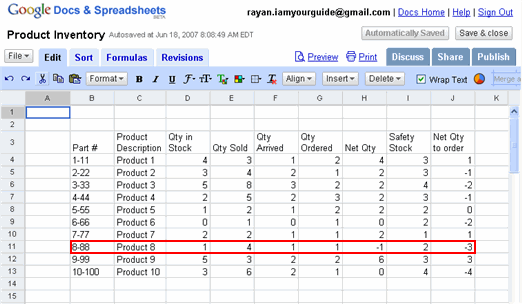
We can test the worksheet for its correctness, by typing in numbers that are easy to calculate with. Luckily in our case the numbers are simple enough to be calculated mentally or using a calculator.
Take for instance the Product 8 with part # 8-88, for which the figures can be read out from the above table and listed as follows :
Qty in Stock = 1
Qty Sold = 4
Qty Arrived = 1
Qty Ordered = 1
and our formula for Net Qty = Qty in Stock – Qty Sold + Qty Arrived + Qty Ordered
Net Qty = 1 – 4 +1 +1 +1 = -1 which is correct as seen from the table.
Next, Safety Stock = 2
and our formula for Net Qty to order = Net Qty – Safety Stock
Net Qty to order = -1 -2 = -3 which is again correct as seen from the table.
Alternatively we can plug in known numbers in the above table for which we know the answer and see if the spreadsheet shows it correctly.
It is also advisable to test the spreadsheet to see if it works in the following special cases:
- what if the cell contain Zero values (this may happen when say we divide a number by another and the denominator happens to be a zero. We need to see if the spreadsheet shows an appropriate error message)
- what if one of the cells go blank in the formula ( this may happen when we copy and paste formula from one cell to a series of cells down below and some cells happen to be blank. Again division of a number with a cell that is empty should lead to an appropriate error message)
- what if the calculated cell contain very large values like 1247828883123 ? For example, this may happen when we multiply two large values like 456789 and 12345. Is the result cell wide enough to show it?
- what if the cell contain very small values? For example, division of a cell value with another containing a very small value like 0.0000000000000000015 should result in a very large number. In such a case, is the result cell wide enough to show it?
Obviously, all of these extreme cases cannot be illustrated in this simple exercise. Don’t you worry, as we go further in our lessons we would know how to handle such problems.
Documentation of worksheet
Before we go to our next session, it is good to know how to document any worksheet. As time goes by, we tend to forget who created it, when it was created and what is its purpose etc.
It is customary to place the documentation worksheet as the first in the group of worksheets, that together make up the workbook. As of now we have just this one sheet, Sheet1, where we have listed the products with stock. It is sheet that is currently active, which we can tell from the way the name of the sheet appears. As we could see, the name Sheet1, is all-white and stands out boldly. Now to add the documentation worksheet, we need to click on the Add Sheet button on the lower left hand corner as shown below.
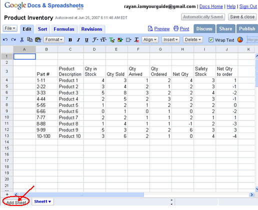
Clicking on this button adds a new sheet,Sheet2 to the right of the existing Sheet1. 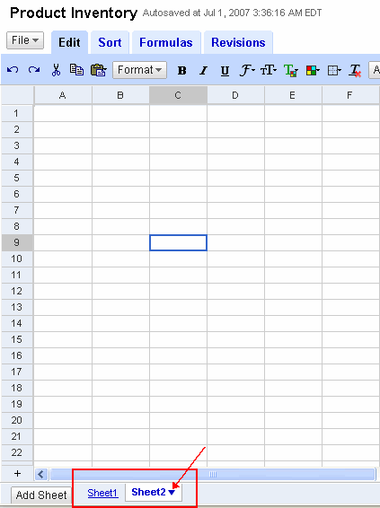
Now this sheet, Sheet2 becomes active and Sheet1 becomes inactive. Again we can tell this from the way the two sheet names appear. Sheet2 is all-white and bold and Sheet1 is grayed out and there appears an hyperlink below it. Notice also that there is a small inverted blue triangle beside the name Sheet2, to show that there is a drop down menu that accompanies it. Now click on it to see the menu options.
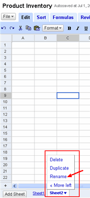
As we could see, there are 4 menu options with this Sheet2: either Delete this sheet, Duplicate it, or Rename it or Move it to the left. First will rename it and then move it to the left of the Sheet1. So first click on Rename.
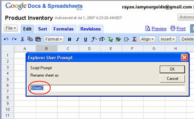
A prompt (explorer user prompt) appears. To rename Sheet2 as Documentation Sheet, type in the highlighted region, “Documentation Sheet” and click OK. Sometimes when we make some changes to the worksheet, it doesn’t happen immediately. That’s because, our requests need to be communicated to the Google Server and executed on the server. So we see a label that appears at the top either as “Updating” or “Trying to reach Google.com” to inform us that the updating is in progress. This is because the server sometime gets busy with too many requests from clients like you and me, and our requests are executed in due time. This is perfectly normal and not to be concerned with.
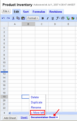
As we could see Sheet2 is now renamed as Documentation Sheet. To make this sheet as the first sheet that anyone sees while opening this workbook, we need to move it to the left. To do this we use this option “<< Move left" as seen above. Click on it to move the Documentation Sheet to the left of the Sheet1.
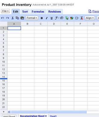
As you could see the Documentation Sheet has moved over to the left and will be the first sheet seen by the user when this workbook is opened. Now we are ready to document the workbook with details that were brought out during the planning phase.
Type in cell D1, the name of the company – Special Products Inc.
in cell B4 – Purpose
in cell B6 – Created By
in cell B8 – Date Created
in cell B10 – Guidelines / Assumptions
as shown below:
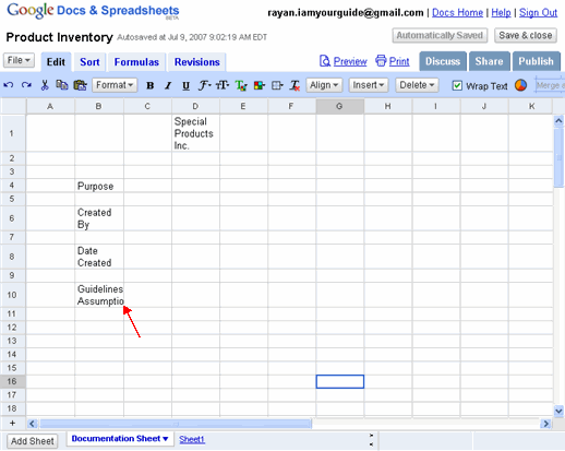
As is shown by the pointer, the cell contents of B10 are not fully visible. Increase the column width of B as told earlier in create a skeleton worksheet.
Also please notice that the contents of cell D1 seems to be somewhat cramped in its location. For this we can increase the column width of D, but a more elegant solution would be to make the contents spread across more than one column, say D through F.
To do this click on cell D1, press & hold Shift key and click on F1 to select all cells D1 through F1
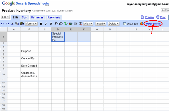
and then click on Merge Across button as shown above.
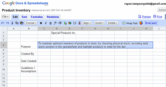
Now click on cell C4, press & hold Shift key and click on K4 to select all cells C4 through K4 and then click on Merge Across button again to merge cells C4 through K4.
Click on cell C4 and type in the following:
To maintain optimum inventory of products in store, by checking physical stock, recording daily stock position in the spreadsheet and highlight products to order for the day
With these changes made the documentation sheet should appear as follows:
Click on cell C10, press & hold Shift key and click on K15 to select all cells C10 through K15 and then click on Merge Across button again to merge cells across columns C through K for rows 10 to 15.
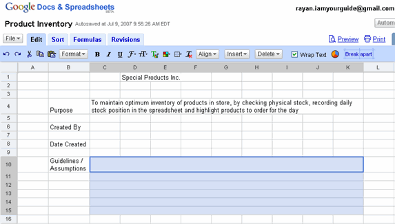
Now the documentation sheet appears as above.
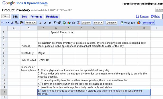
To complete the documentation, type in the following in the respective cells:
Cell C6: Your name
Cell C8: Today’s date
Cell C10: 1. Check physical stock and update the spreadsheet every day.
Cell C11: 2. Place order only when the net quantity to order turns negative and the quantitiy to order is the negative quantity.
Cell C12: 3. If the net quantity to order is either zero or positive, there is no need to order.
Cell C13: 4.To save on shipping bunch orders together as much as possible.
Cell C14: 5. Lead time for orders with suppliers fairly predictable and stable.
Cell C15: 6.There are no damage to goods in transit / storage and there are no rejects in consignment received.
Now the completed documentation sheet should look as follows:
In the next section we will see as to how to format the cell contents to make this workbook look professional and presentable.
<--BackTo: Fillup the worksheet
Next: Format the worksheet I –>